Cutting CFD Turnaround with Upfront Sanity Checks

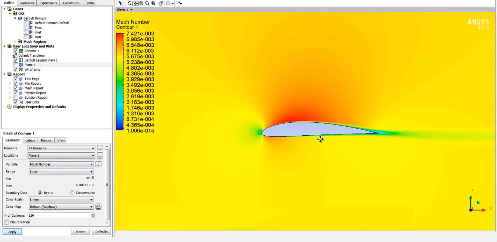
The Need for Minimal Upfront Sanity Checks in CFD

In aerodynamic analysis, a full CFD workflow is typically time-consuming: selecting an airfoil section, building fluid domain CAD geometry, generating spatial volume meshes, setting up boundary conditions and turbulence models, and submitting RANS simulations to the solver. A single run can easily take hours, and with 3D vehicle geometries or fine meshes, it often takes several days to obtain converged flow fields and aerodynamic force coefficients. On modest hardware, this waiting time is even more noticeable.

Long compute times are an accepted engineering trade-off, but discovering after days of computation that the initial setup contained an inverted sign is deeply frustrating. Common setup errors include reversing coordinate axes, flipping angle-of-attack signs (computing unintended lift instead of downforce), misinterpreting chord scaling, or introducing surface curvature discontinuities that degrade mesh quality or trigger divergence. These avoidable mistakes waste both compute resources and engineering time.

The motivation was clear: before launching an expensive, long-running CFD computation, can a low-cost, millisecond-scale method serve as an upfront sanity check to catch obvious mistakes? It does not need multi-decimal precision, but it must instantly confirm three essentials:

1. Is the sign and direction of lift correct?
2. Are the order of magnitude of lift and aerodynamic loads reasonable?
3. Where is the suction peak located, and is the geometry orientation flipped?

This article outlines how I designed this low-cost sanity-check workflow and provides a Python demo.

Implementing Two Classical Inviscid Methods

To keep the sanity checks lightweight, I implemented two classical inviscid potential flow methods in the Python demo:

1. Thin-Airfoil Theory: Flattens the airfoil into a zero-thickness camber line, providing a closed-form formula $C_l = 2\pi\alpha$ to instantly estimate lift;
2. Hess–Smith Panel Method: Discretizes the true outer contour of the airfoil into straight line segments with distributed source and vortex strengths, calculating both integrated lift and surface pressure coefficient ($C_p$) distributions.

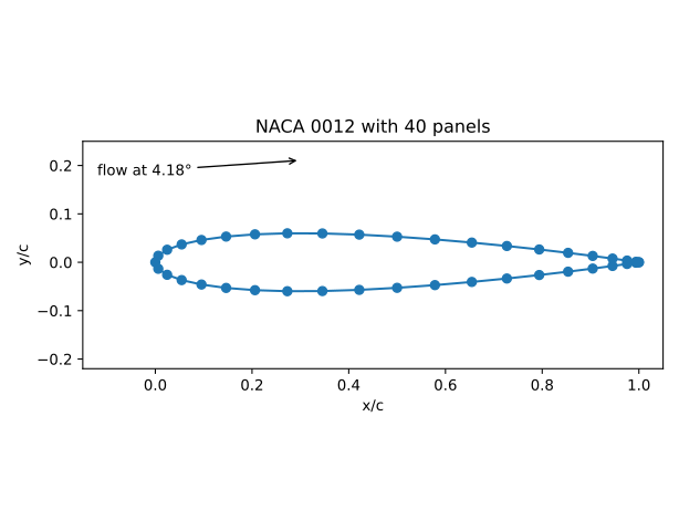
The diagram illustrates the geometric discretization in the panel method: a smooth airfoil profile is discretized into interconnected line segments, with cosine spacing applied to refine resolution near the leading and trailing edges where curvature varies rapidly. After implementing this demo, key verification questions arose: how reliable are these estimates, to what degree can we trust the output, and under what conditions do they break down? To address this, I benchmarked against wind-tunnel experimental data for the classical symmetric NACA 0012 airfoil from NASA TM-4074.

Evaluating a Baseline Case at 4.18° Angle of Attack

Before detailing the numerical formulation, consider a single operating point: the airfoil at a small angle of attack $\alpha = 4.18^\circ$, comparing the demo’s predictions against NASA wind-tunnel measurements. The NACA 0012 is a standard symmetric airfoil (00 denotes zero camber; 12 indicates a maximum thickness of 12% chord). All comparisons are evaluated at Mach number $M=0.15$ (the NASA test conditions correspond to Reynolds number $Re=5.97\times10^6$ with free boundary-layer transition).

Lift Prediction at $\alpha=4.18^\circ$	Lift Coefficient $C_l$	Relative Error vs. NASA Test
NASA Wind Tunnel (Ladson TM-4074)	0.4520	—
Thin-Airfoil Theory (1-line formula + compressibility correction)	0.4636	+2.6%
Hess–Smith Panel Method (160 panels + compressibility correction)	0.5096	+12.8%

The lift coefficient $C_l$ is a non-dimensional quantity that normalizes out fluid density, velocity, and reference area:

$$L=\frac{1}{2}\rho V^2 S C_l.$$

Non-dimensional scaling allows direct comparison among simplified formulas, numerical models, and wind-tunnel experiments on a common basis. This comparison reveals an interesting observation: thin-airfoil theory, which uses a single equation and completely neglects thickness, has an error of only 2.6%; meanwhile, the panel method, which discretizes the full 12% thickness profile across 160 panels, shows a larger error of 12.8%. Why does the seemingly more refined panel method yield a higher total lift error? Why bother with the panel method at all? Such counterintuitive behaviors are common in aerodynamic modeling. Thin-airfoil theory provides only a single scalar lift value, whereas the panel method computes the full surface pressure distribution.

NASA Wind-Tunnel Benchmark Data

To establish reliable ground truth, I referenced Charles L. Ladson’s experimental report, NASA TM-4074, conducted in the NASA Langley Low-Turbulence Pressure Tunnel (LTPT).

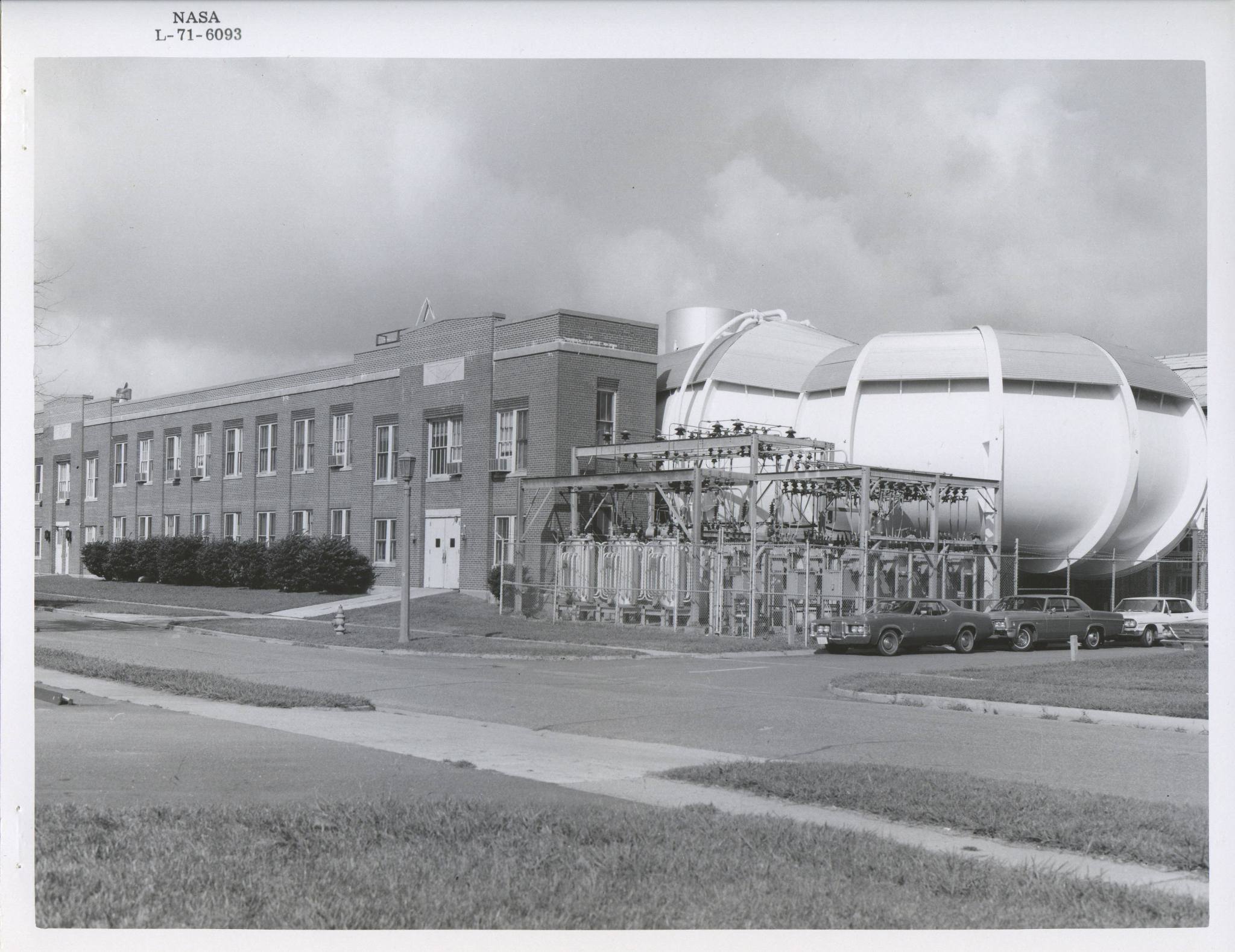
This pressurized facility enabled independent variation of Mach and Reynolds numbers without altering gas composition, providing a low-turbulence, well-controlled experimental environment.

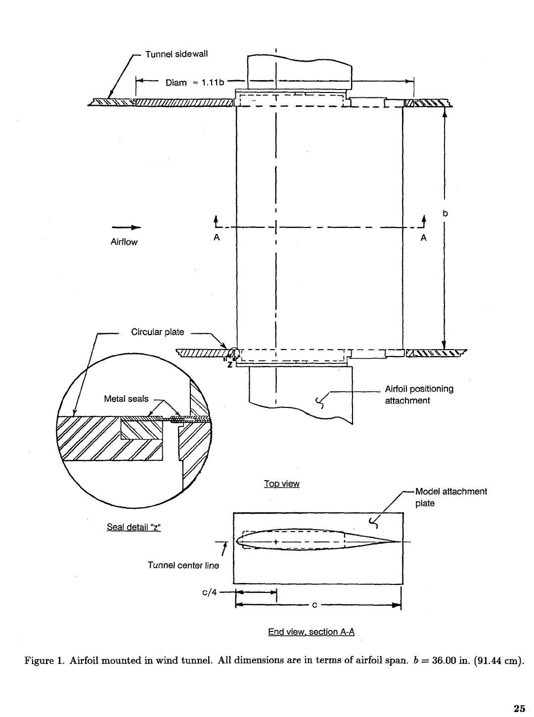
The test model spanned the entire test section with a chord of 23.66 inches and 81 surface pressure orifices. Lift and pitching moment were obtained by integrating surface pressure tap measurements, while drag was determined using a downstream wake survey rake.

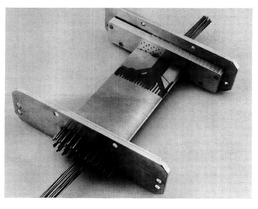
The photograph shows the wind-tunnel model: small orifices near mid-span measure surface pressure, connected via internal metal tubing to pressure transducers. NASA reported zero-angle repeatability within $\Delta C_d \le 0.0002$ and normal force coefficient repeatability within 0.004. I extracted the free-transition dataset at $M=0.15$ and $Re=5.97\times10^6$ spanning 16 angles of attack from $-4.05^\circ$ to $17.35^\circ$ as the validation benchmark.

Thin-Airfoil Theory

For symmetric airfoils, thin-airfoil theory gives a clean closed-form lift relation:

$$C_l = 2\pi\alpha,$$

where $\alpha$ is in radians. In degrees, the theoretical lift curve slope is approximately $0.1097/\text{deg}$. At $\alpha = 4.18^\circ$ ($\approx 0.07295\ \text{rad}$), the incompressible lift coefficient is 0.4584. Applying the Prandtl–Glauert subsonic compressibility correction factor $1/\sqrt{1-M^2} \approx 1.0114$ at $M=0.15$ gives an estimated $C_l = 0.4636$.

This approach reduces the airfoil to a zero-thickness mean camber line. It does not account for profile thickness, surface suction distributions, profile drag, or stall characteristics. However, its value lies in immediate evaluation—confirming lift direction and order of magnitude without computational delay.

Hess–Smith Panel Method: Resolving Surface Pressure Distributions

When surface suction peak locations, geometric curvature, or upper/lower surface orientation need verification, the physical geometry must be retained. This is where the Hess–Smith panel method applies. The airfoil contour is discretized into 160 panel segments:

1. No-Penetration Boundary Condition: At each panel midpoint (control point), the normal velocity component is enforced to zero, forming the source influence matrix;
2. Circulation & Kutta Condition: A uniform vortex strength is applied across all panels, enforcing smooth flow departure at the trailing edge to satisfy the physical Kutta condition and establish circulation;
3. Linear System Solution: Solving the coupled linear equations yields source strengths and total circulation, from which tangential surface velocities $V_t$ are computed;
4. Pressure Coefficient Calculation:

$$C_p = 1 - \left(\frac{V_t}{V_\infty}\right)^2.$$

More negative $C_p$ values indicate higher local flow velocities and stronger static pressure suction. Integrating this pressure distribution over the closed contour yields the lift coefficient, inviscid pressure drag, and pitching moment.

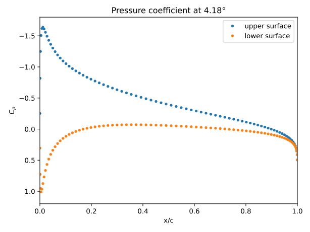
In standard aerodynamic plotting conventions, the vertical $C_p$ axis is inverted (negative suction values upward). The plot clearly displays a prominent suction peak near the upper surface leading edge under positive angle of attack, balanced by positive pressure along the lower surface. This illustrates the primary utility of the panel method: while more involved than a single-line formula, it provides immediate insight into the physical flow field.

Mesh Convergence Verification

Before benchmarking against NASA measurements, numerical code implementation errors must be ruled out through verification:

1. Geometry and Zero-Angle Symmetry: At $\alpha = 0^\circ$, symmetric airfoil lift evaluates to exactly zero, and upper/lower surface pressure distributions overlap identically;
2. Near-Zero Pressure Drag: Inviscid 2D potential flow theoretically produces zero pressure drag; integrated pressure drag evaluates to the order of $10^{-4}$, confirming numerical consistency;
3. Panel Refinement Study: Panel resolution was scaled across 40, 80, 160, and 240 panels.

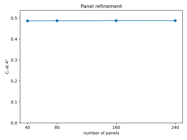
At $\alpha = 4^\circ$, panel counts of 40, 80, 160, and 240 produced $C_l$ values of 0.48646, 0.48727, 0.48773, and 0.48788, respectively. Increasing from 160 to 240 panels changed lift by only 0.0307%. This confirms mesh convergence: discrepancies against experimental data stem from the underlying physical assumptions rather than spatial discretization errors.

Key Insights and Methodological Observations

Several engineering insights emerged during this study:

1. Geometric Detail Does Not Always Mean Higher Total Lift Accuracy, but Resolves Flow Topology

Across the linear range ($-4.1^\circ \le \alpha \le 10.2^\circ$), the fitted lift slope comparisons are summarized below:

Linear Regime Comparison ($-4.1^\circ \sim 10.2^\circ$)	NASA Experimental	Thin-Airfoil + Correction	Hess–Smith Panel + Correction
Lift Curve Slope (per degree)	0.10684	0.11092	0.12162
Relative Slope Error	—	+3.81%	+13.83%
Linear Range $C_l$ RMSE	—	0.0226	0.0824

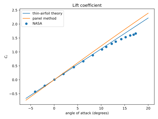
Why does the panel method, which includes profile thickness, overestimate total lift relative to thin-airfoil theory?

• Inviscid Physical Mechanism: Inviscid potential flow assumes zero fluid viscosity; flow acceleration over a thickened upper surface is stronger than over a flat plate, generating greater circulation under an ideal Kutta condition;
• Viscous Real-World Effects: In real viscous flows, boundary-layer growth thickens toward the trailing edge, reducing effective camber and trailing-edge sharpness (boundary layer displacement softens the effective Kutta condition, reducing circulation);
• Thin-Airfoil Error Cancellation: Thin-airfoil theory neglects thickness-induced acceleration. This omission partially cancels the overestimation from neglecting viscous decambering, yielding an integrated lift value that coincidentally matches experiment more closely.

However, the panel method remains essential: it provides full surface pressure distributions, enabling quick visual verification of suction peaks, orientation, and sign convention before running CFD—capabilities thin-airfoil theory cannot provide.

2. Breakdown at High Angles of Attack: Separation and Stall

At $\alpha = 17.35^\circ$, the measured NASA lift coefficient is 1.660, exhibiting clear non-linear stall curvature. In contrast, the panel method continues along a linear slope to 2.085 (full-range RMSE increases to 0.225). This highlights a fundamental limitation of inviscid flow: lacking viscous dissipation terms from the Navier–Stokes equations, it cannot capture boundary-layer separation or aerodynamic stall. Potential flow methods cannot evaluate high-incidence or post-stall regimes.

3. Near-Zero Drag Prediction: d’Alembert’s Paradox

The method’s physical limitations are most apparent in drag estimation.

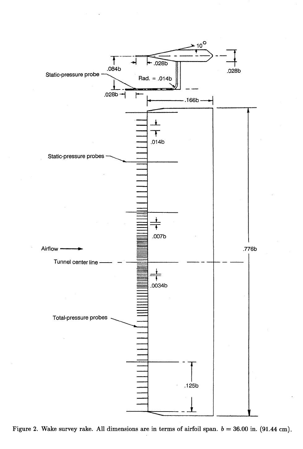
NASA experimentally determined aerodynamic drag via downstream momentum deficit measurements with a wake rake, recording baseline profile drag of $C_d \approx 0.0065$ near zero angle of attack, increasing to 0.0275 at $17.35^\circ$.

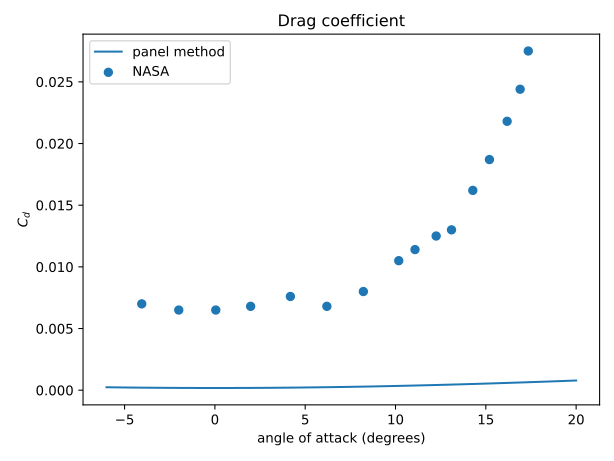
The panel method’s integrated pressure drag remains below 0.0008 across all angles. This reflects d’Alembert’s Paradox: in steady 2D inviscid potential flow around a closed body, the net pressure drag is identically zero. The non-zero values computed by the panel method represent numerical integration truncation errors.

Code

The solver implementation and validation scripts are open-source on GitHub: gaoflow/airfoil-methods

git clone https://github.com/gaoflow/airfoil-methods.git
cd airfoil-methods
python3 -m unittest discover -s tests -v
python3 scripts/analyse.py

Running the analysis script executes all geometric verifications, aerodynamic comparisons, and regenerates all figures shown above.

References

1. Charles L. Ladson, Effects of Independent Variation of Mach and Reynolds Numbers on the Low-Speed Aerodynamic Characteristics of the NACA 0012 Airfoil Section, NASA TM-4074, 1988. The 16-point lift and drag validation dataset and experimental conditions are drawn from Table I.
2. J. L. Hess & A. M. O. Smith, Calculation of Potential Flow About Arbitrary Bodies, Progress in Aerospace Sciences, volume 8, 1967, pages 1–138. Foundation reference for surface source and vortex panel methods.