Comparative Analysis of Fluent Results Against Exact Solutions, Meshes, and Experimental Data
Verifying Fluent pipe flow calculations against the Poiseuille exact solution, followed by mesh, domain, and Re=0.1–20 sweeps for flow past a cylinder compared with experimental data.
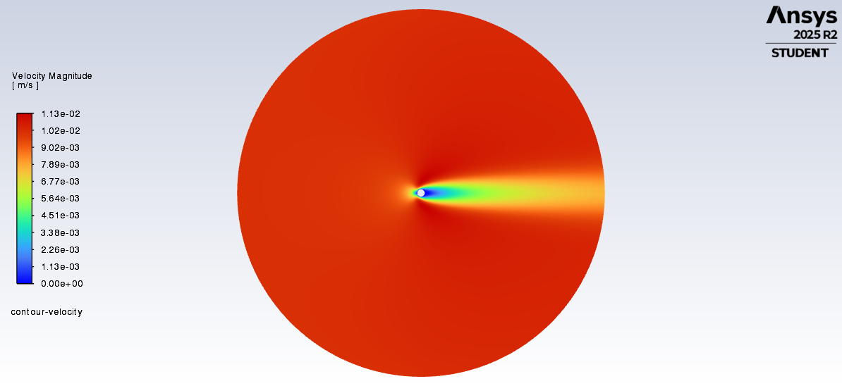
This is my lab record from the Computational Fluid Dynamics course in the Spring 2026 semester.
Course Requirements
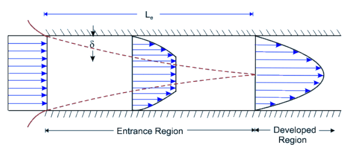
The assignment first gave us a pipe 10 m in length and 0.4 m in diameter: fluid enters at a uniform velocity of 1 m/s and gradually evolves into fully developed flow under wall friction. The instructor required us to first calculate the Reynolds number and the analytical hydrodynamic entrance length to determine whether the pipe is long enough; then examine convergence, mass conservation, velocity profiles, wall shear stress, and pressure drop, ultimately comparing the results against the exact Poiseuille solution. The course schematic illustrates this process straightforwardly: boundary layers along both walls thicken from the inlet, merge at the end of the entrance region, and thereafter maintain a parabolic velocity profile. This serves as an excellent foundational case for learning CFD.
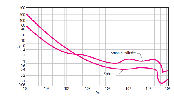
The flow past a cylinder task transitioned the problem to an external flow lacking a closed-form analytical solution: the outer boundary must be sufficiently far, the cylinder boundary and the entire domain require defined mesh resolutions, and the simulation results must be checked for convergence, mass conservation, flow fields, and drag, followed by comparison against the smooth cylinder drag curve provided in the course.
Next, I used pipe flow with its exact analytical solution to calibrate the simulation workflow, before switching to flow past a cylinder to systematically examine mesh sensitivity, domain sizing, and experimental discrepancies. This prompted a fundamental question: are the numbers output by Fluent truly reliable?
Calibrating the Workflow with Pipe Flow
The pipe has a length of 10 m and a radius of 0.2 m, with an inlet mean velocity of 1 m/s, density of 1 kg/m³, and dynamic viscosity of 0.004 Pa·s, yielding . In Fluent, I used a mesh of 500 quadrilateral cells and 561 nodes. The comparison results are as follows:
| Check / Metric | Analytical Value | Fluent Result |
|---|---|---|
| Convergence | Residuals | Reached at iteration 53 |
| Mass imbalance | 0 | kg/s |
| Maximum centerline velocity | 2.00 m/s | 1.98 m/s |
| Wall shear stress | 0.08 Pa | 0.08 Pa |
| Fully developed pressure drop | 8 Pa | 8.65 Pa |
| Entrance length | 2.4 m | m |
First, let us examine the velocity field to verify whether the uniform inflow genuinely evolves into a Poiseuille parabolic profile.
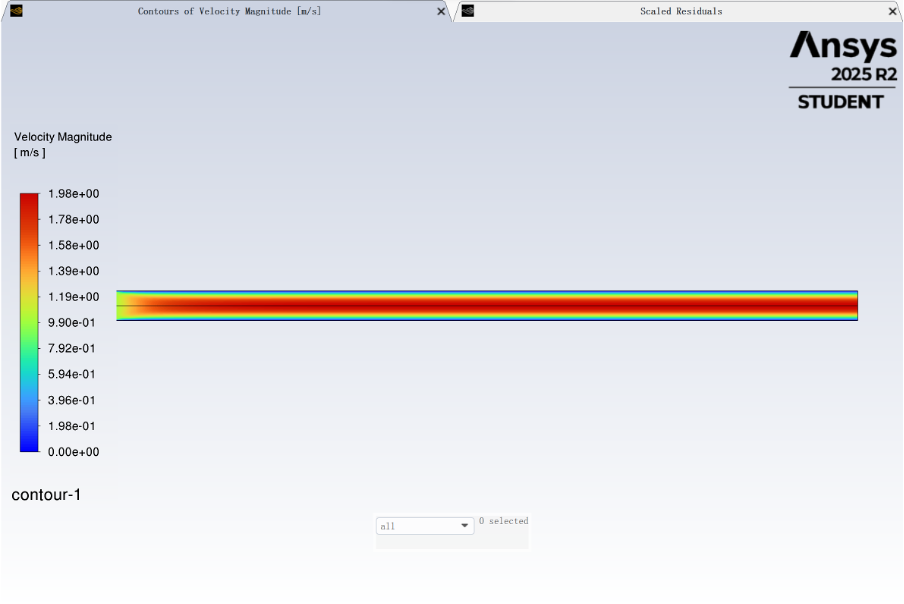
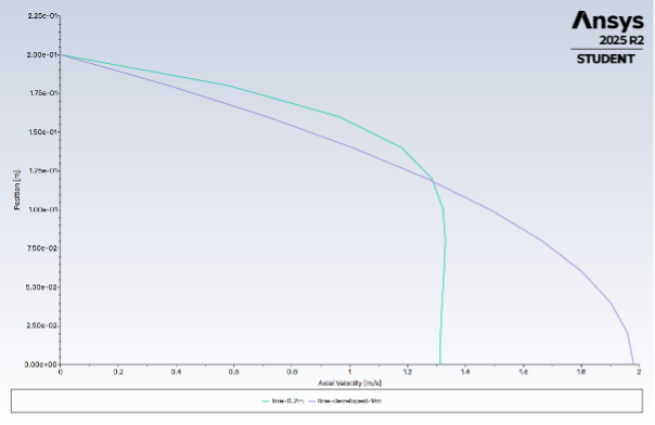
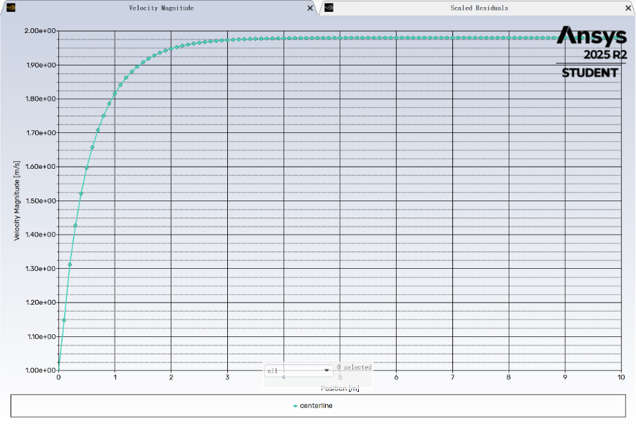
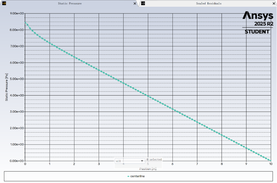
The centerline velocity shows a 1% difference. The extra 0.65 Pa in pressure drop originates from the entrance region: before the velocity profile fully develops into a parabola, the velocity gradient at the wall is steeper, naturally producing higher wall friction. Visually from the plot, the entrance region spans roughly 2 m. When evaluated where the centerline velocity reaches 99% of its asymptotic value, the length is approximately 2.4 m, consistent with analytical correlations.
Investigating the Cylinder Case Without an Exact Solution
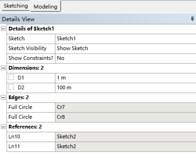
The cylinder diameter is 1 m, surrounded by a circular external domain of diameter . The density is 1 kg/m³ and dynamic viscosity is Pa·s; Reynolds numbers are varied by adjusting the inlet velocity. The setup is 2D, steady, laminar, and incompressible. A uniform velocity is prescribed at the inlet, zero gauge pressure at the outlet, and no-slip at the cylinder wall.
I first identified the grid and domain independence plateaus at , then locked these settings to sweep from to 20.
| Cell Count | 50 | 200 | 450 | 800 | 12,800 | 28,800 | 40,000 |
|---|---|---|---|---|---|---|---|
| 3.1328 | 2.7982 | 2.7757 | 2.7800 | 2.7938 | 2.7953 | 2.7973 |
Starting from 12,800 cells, the variation in remains below 0.1%. I ultimately selected 40,000 cells with .
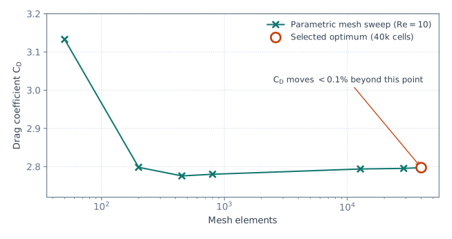
Notably, refining from 12,800 to 28,800 cells produced a variation of only 0.05%, with the two points lying very close together. However, two adjacent fine-mesh points alone do not prove the existence of an asymptotic plateau—they might simply happen to be near each other before convergence. Therefore, I also swept in the coarser direction. The 50-cell mesh yielded 3.1328, approximately 12% higher than the converged value. It is precisely this coarse-grid anchor that demonstrates the solution genuinely varies with resolution, making the direction and magnitude of grid dependence visible and truly convincing.
With the mesh fixed, I increased the outer domain diameter from 100 m to 200 m:
| 100 m | 120 m | 150 m | 180 m | 200 m | |
|---|---|---|---|---|---|
| 2.7973 | 2.7889 | 2.7806 | 2.7751 | 2.7723 |
The variation from 100 m to 200 m is under 1%, so 100 m was retained.
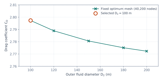
Smaller domains of 20–80 m elevated to approximately 3.05, indicating that tight outer boundaries artificially constrict the flow. However, because those lower domain points also used coarser boundary discretizations, they only demonstrate the order of magnitude of domain confinement without fully isolating domain size from mesh density.
The parametric sweep employed a consistent mesh of ~20,200 nodes with m. As increased from 0.1 to 20, dropped from 92.4 to 2.06.
| Inlet Velocity (m/s) | Drag Force (N) | ||
|---|---|---|---|
| 0.1 | 92.4 | ||
| 0.5 | 19.37 | ||
| 1 | 11.43 | ||
| 5 | 4.11 | ||
| 10 | 2.85 | ||
| 20 | 2.06 |
The two animations below sequentially display actual Fluent outputs across , 0.5, 1, 5, 10, and 20.
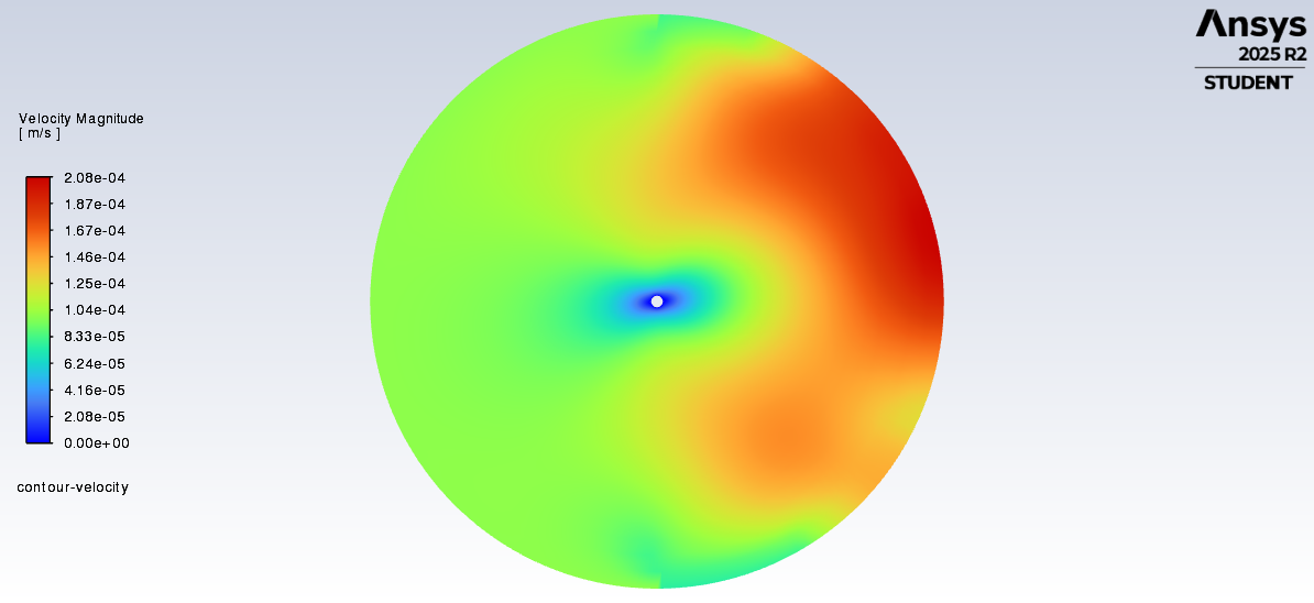
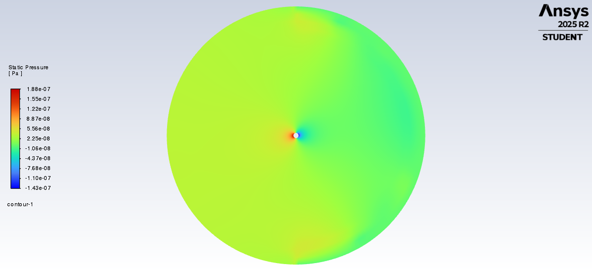
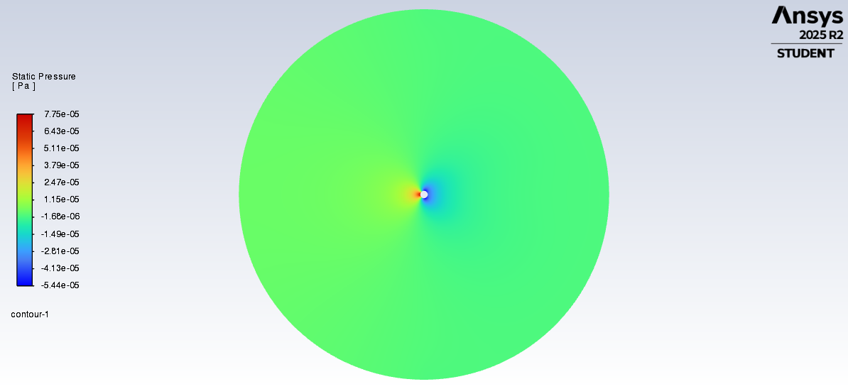
The endpoint contour comparisons highlight the structural differences across the sweep. At , viscous effects diffuse over an extensive region, leaving only a smooth, symmetric low-velocity zone behind the cylinder; by , the wake becomes noticeably more concentrated, and both the upstream stagnation high pressure and downstream low-pressure wake are clearly defined.
Comparison with Six Experimental Cases
Comparing against the experimental table from the course notes, only fell within the 5% error margin:
| 0.1 | 0.5 | 1 | 5 | 10 | 20 | |
|---|---|---|---|---|---|---|
| Relative Error | 81.2% | 51.1% | 48.9% | 32.4% | 17.5% | 3.83% |
The other five operating points failed the criterion :(
Why was the discrepancy largest at very low Reynolds numbers? In post-analysis, one contributing factor is setup configuration: the sweep mesh was coarser than the 40,000-cell reference grid at , and the domain was smaller. These setup differences alone shifted at from 2.7973 to 2.85. Another potential reason stems from model assumptions: at , steady 2D flow is a much more demanding assumption. In the run, continuity residuals stalled, and velocity residuals only dropped to ; consequently, the 92.4 drag coefficient is the least reliable among the six results.
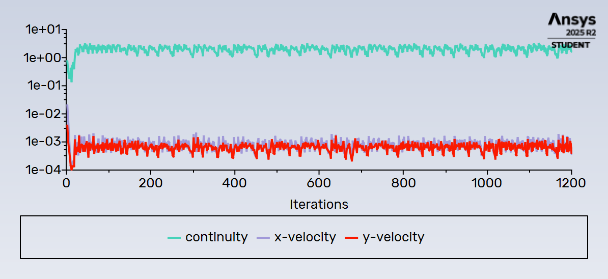
The written documentation for the pipe flow noted a 1,000-cell mesh, but the only surviving console log originated from a 500-cell run. This article reports data aligned with that log. Another discrepancy surfaced in the cylinder surface pressure coefficient () curves: the exported plot labeled was identical to the file. As a result, this article excludes that plot from supporting conclusions for . The static pressure contour and force data table for correctly correspond to that condition. Hence, every figure and number must first be traced back to its specific run provenance; filenames and captions are merely clues, whereas console logs and raw outputs establish true data attribution.
Summary
This assignment served as the starting point for establishing my CFD verification and validation methodology. I began with two relatively simple steady-state problems: verifying pipe flow against the exact Poiseuille solution, followed by examining low-Reynolds-number cylinder flow across varying meshes, domain sizes, and external reference benchmarks. This stage addressed a fundamental question: what rigorous checks must a steady CFD result undergo before it can be trusted?
Establishing a mesh independence plateau cannot rely solely on two closely agreeing fine-grid points. One must also sweep toward coarser meshes to observe the solution clearly diverging from the plateau; computational domain size must likewise be varied independently to verify that far-field boundaries no longer artificially constrain drag. Among the six Reynolds number cases, only met the 5% error threshold. This demonstrates that residual convergence is merely a starting prerequisite—it does not inherently guarantee that the model, mesh, and computational domain are sufficiently accurate.
The investigation here concluded with 2D steady laminar flow at . Having established this systematic verification protocol, I subsequently extended the cylinder case to higher Reynolds numbers in subsequent assignments: first establishing a steady wake benchmark at , and then investigating unsteady vortex shedding, lift/drag histories, and the Strouhal number at . The logical progression is clear: first confirm whether steady-state results are credible, and only then investigate how flow dynamics evolve over time.