From Melting Snow to a 2D Heat Diffusion Solver

Observing Snow on Cobblestones

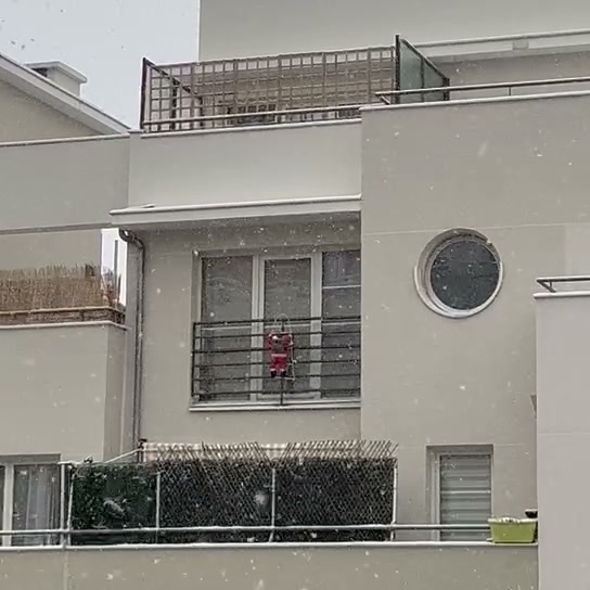
During several heavy snowfalls in Paris, while spacing out and watching the snow on cobblestone pavements one day, I noticed a fascinating pattern: snow on top of paving stones often melted faster than on the surrounding soil, sometimes even tracing the exact outline of each brick. Looking into the reason, I found it stemmed from the thermal conductivity difference between stone and soil—subsurface ground heat conducts upward through masonry bricks faster, creating temperature gradients across the snow layer.

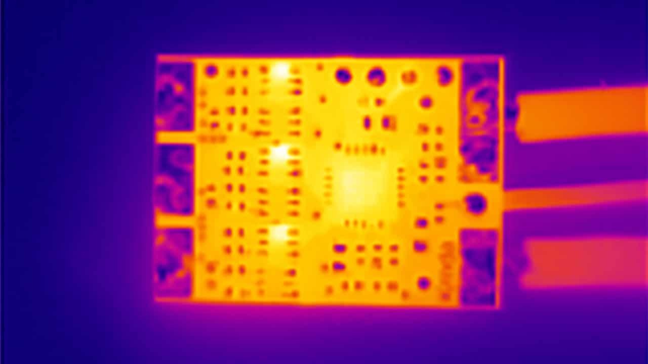
I found this mechanism intriguing, and realized it also appears in various engineering scenarios: vapor chambers beneath semiconductor chips or cooling baseplates in battery packs, where local heat sources concentrate energy before solid-state conduction spreads it out. However, actual snow melting involves latent heat of fusion, uneven snowpack thickness, and complex material interfaces—too many coupled variables for an initial study. So I simplified it into a cleaner problem: a 2D metal plate cooled from one side.

Simplified Model: A Metal Plate Cooled on One Side

The simplified model of the snow problem is as follows: a 2D metal plate with an initial uniform temperature $T=1$. At $t=0$, a cold source at constant temperature $T=0$ is applied to the left boundary, while the remaining three edges are perfectly insulated. Internal heat can only escape through this single channel on the left.

I also non-dimensionalized the formulation so the results can scale proportionally to any real-world operating condition. This model preserves the core physics of the snow problem—heat diffusing through a solid over time to smooth out temperature variations—while stripping away latent heat, complex geometry, and material interfaces. Crucially, it possesses an exact Fourier series analytical solution, allowing numerical results to be audited point by point at any time.

Running into Solver Instability

I wrote a 2D explicit Forward-Time Central-Space (FTCS) heat diffusion solver to observe how the internal temperature field evolves over time when the plate is cooled from one side. Initially, the program ran smoothly. To speed up computation, I casually bumped up the time step $\Delta t$ slightly. For the first few dozen steps, the temperature contour looked smooth and natural, and the cooling process appeared completely plausible. But just a few dozen steps later, the entire numerical matrix collapsed within a handful of iterations, flooding the screen with NaNs.

This got me thinking: before blowing up, the solver produced dozens of seemingly normal, smooth illusions. If a numerical algorithm does not immediately flag an error before heading toward catastrophic divergence, how do we know in more complex engineering setups whether the contours we see are correct or secretly collapsing? To understand why a time-dependent solver can suddenly spin out of control, how to reject dangerous parameters before execution, and how to isolate temporal accuracy amidst mixed discretization errors, I began this investigation.

1. Problem Analysis

I first returned to the 2D heat diffusion equation and its discretization:

$$\frac{\partial T}{\partial t} = \alpha \left( \frac{\partial^2 T}{\partial x^2} + \frac{\partial^2 T}{\partial y^2} \right)$$

On a square grid ($\Delta x = \Delta y$), the algebraic update scheme for Forward-Time Central-Space (FTCS) is:

$$T_{j,i}^{n+1} = T_{j,i}^{n} + r \left[ (T_{j,i+1}^{n} - 2T_{j,i}^{n} + T_{j,i-1}^{n}) + (T_{j+1,i}^{n} - 2T_{j,i}^{n} + T_{j-1,i}^{n}) \right]$$

where the dimensionless diffusion number $r$ is:

$$r = \frac{\alpha \Delta t}{\Delta x^2}$$

Why did increasing the time step cause the program to blow up? Through Von Neumann stability analysis, decomposing spatial numerical error of arbitrary wavelength into Fourier modes yields the single-step amplification factor $g$:

$$g = 1 - 4r \left[ \sin^2\left(\frac{k_x \Delta x}{2}\right) + \sin^2\left(\frac{k_y \Delta x}{2}\right) \right]$$

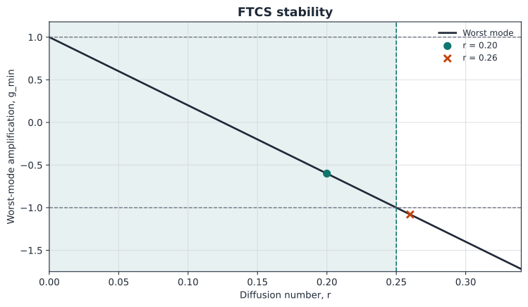
To ensure numerical stability, all spatial modes must satisfy $|g| \le 1$. The most dangerous and easily excited mode is the highest-frequency sawtooth oscillation at the grid scale (where adjacent nodes alternate phase, $\sin^2 = 1$). Substituting this limiting case yields the worst-mode amplification factor:

$$g_{\text{worst}} = 1 - 8r$$

Enforcing $g_{\text{worst}} \ge -1$ leads directly to the strict stability criterion for the 2D explicit FTCS scheme:

$$r \le 0.25$$

This explains the root cause of the collapse: $r \le 0.25$ is a strict numerical stability threshold. Once the time step is slightly oversized such that $r$ becomes 0.26, high-frequency numerical noise is multiplied at every step by an amplification factor greater than 1 in magnitude ($|g| = 1.08$).

Why did the first dozens of steps appear smooth? Because initial floating-point round-off noise is tiny ($\approx 10^{-16}$). Even when multiplied by 1.08 per step, at step 50 the noise is still only on the order of $10^{-14}$, completely masked by the smooth macro-solution. But under exponential growth, by step 100+ the noise rapidly scales to the magnitude of the main solution and overflows to NaN within the next few iterations.

2. Literature Review & Investigation

Having identified the theoretical root cause, I researched literature and industry best practices focusing on two key questions:

First, how do production-grade solvers handle stability boundaries? Reviewing computational heat transfer and CFD literature revealed that many educational scripts either lack guardrails and let calculations diverge silently, or merely print a console warning and continue. In automated pipelines, this allows corrupt data to propagate downstream. Robust software must enforce defensive preconditions before computation begins.

Second, how can the first-order temporal accuracy ($\mathcal{O}(\Delta t)$) be isolated and verified? I initially thought of varying $\Delta t$ on a fixed spatial mesh and taking differences against the Fourier analytical solution to measure convergence order. However, examining the truncation error derivation for FTCS revealed its leading local truncation error:

$$\tau = \frac{\alpha \Delta x^2}{12}(6r - 1) \frac{\partial^4 T}{\partial x^4} + \mathcal{O}(\Delta t^2) + \mathcal{O}(\Delta x^4)$$

The coefficient $(6r - 1)$ of the leading term is directly tied to the diffusion number $r = \alpha \Delta t / \Delta x^2$. When changing $\Delta t$ on a fixed grid, $r$ changes as well, causing the spatial discretization error to fluctuate wildly. If compared directly against a pure mathematical analytical solution, the resulting total error mixes temporal and spatial components, obscuring the true temporal convergence order.

The standard solution from literature is: run a high-precision benchmark on the exact same spatial grid with an ultra-small time step, and compare test cases against this benchmark to cancel out spatial errors completely.

3. Implementation & Solutions

Based on the analysis and findings, I implemented several enhancements: guard against unstable inputs before execution, enforce conservative energy balance structurally in code, and verify temporal convergence orders rigorously against analytical solutions and same-grid benchmarks.

Rejecting Unsafe Time Steps at Launch

Knowing the $r \le 0.25$ threshold, the cleanest approach is preventing non-compliant computations from ever starting. Upon receiving the mesh and time step, the solver calculates $r$. If $r > 0.25$ (e.g., 0.26), it immediately raises StabilityError, records the reason, and terminates without advancing a single step. Warnings are easily overlooked; debugging after several hundred steps turn into NaNs is far too late.

Finite-Volume Flux Balancing for Energy Conservation

I discovered a subtler issue: simulations that look smooth can still secretly leak energy across boundaries. My solution treats each grid cell like a small room, tracking temperature changes purely through heat flux across its four walls. The heat exiting one wall is exactly what the neighboring cell absorbs, meaning all internal fluxes cancel out when summed across the domain. Code structured this way prevents artificial energy leaks. In practice: running 576 steps on a fully insulated domain yielded a total energy drift of exactly 0.0.

Verification & Validation

To confirm solver accuracy, I implemented a suite of 13 unit and verification tests.

First, benchmarking against the analytical standard. On a $1 \times 0.2$ plate ($100 \times 20$ grid), with left boundary $T=0$, remaining three edges insulated, initial $T=1$, and safe $r = 0.20$ ($\Delta t = 2 \times 10^{-5}\text{ s}$), I advanced 2,500 steps to $t = 0.05\text{ s}$ and compared results point by point with the Fourier series analytical solution.

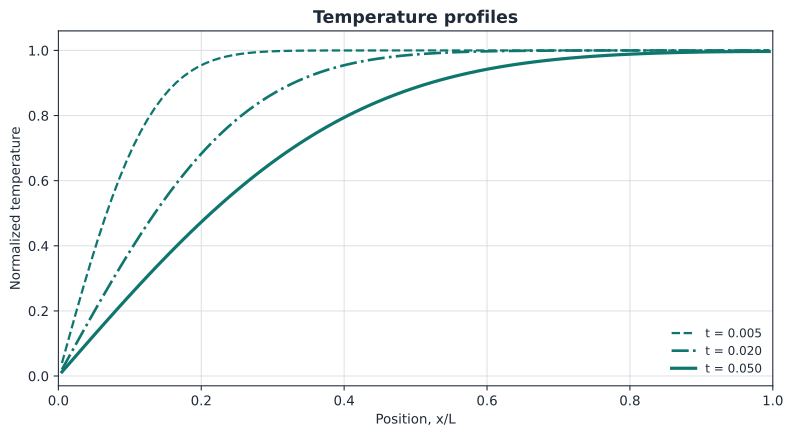
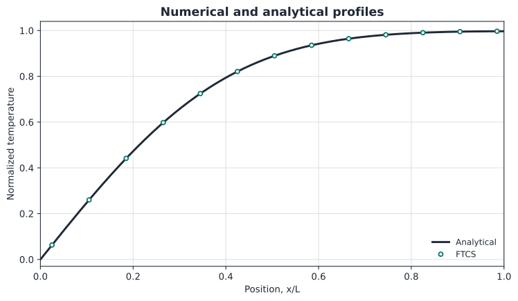
The maximum absolute error was $1.384 \times 10^{-5}$, well below the predefined threshold of $5 \times 10^{-5}$. The transverse temperature difference across the 20 grid rows remained strictly 0.

Next, comparing against a high-resolution benchmark on the same mesh. As analyzed earlier, direct comparison with the analytical solution mixes spatial and temporal truncation errors. Therefore, I first computed a high-precision benchmark on the same grid using $r = 0.001$, then ran four test cases with $r = 0.20, 0.10, 0.05, 0.025$. Subtracting the benchmark cancelled spatial errors, leaving only pure temporal discretization error.

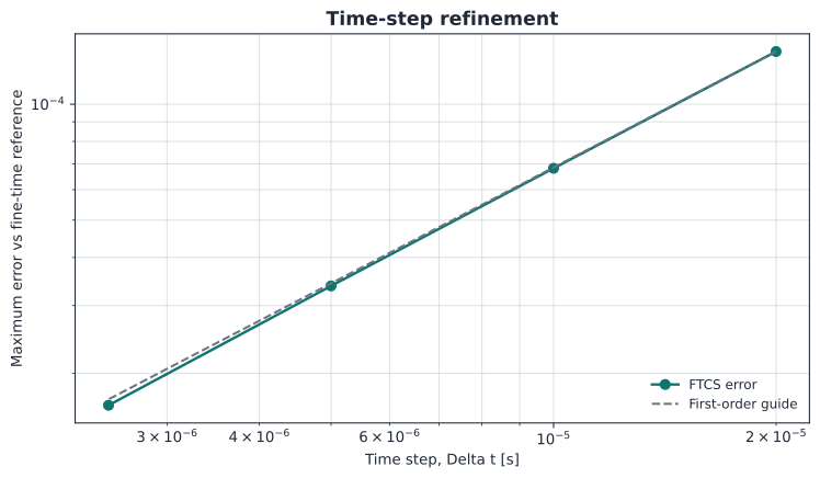
With each halving of the time step, the errors were $1.370 \times 10^{-4}$, $6.817 \times 10^{-5}$, $3.374 \times 10^{-5}$, and $1.653 \times 10^{-5}$—halving consistently each time. The fitted temporal convergence order was 1.017, falling squarely within the theoretical expected range of 0.9–1.1.

Verification Item	Measured Result	Acceptance Criterion	Status
Max absolute error vs. Fourier analytical solution	$L^\infty = 1.384 \times 10^{-5}$	$\le 5 \times 10^{-5}$	Pass
Temporal convergence order on fixed mesh	1.017	0.9 – 1.1	Pass
Discrete energy drift on fully insulated mesh	0.0	$\le 10^{-12}$	Pass
Unsafe time step test ($r = 0.26$)	Raised StabilityError with diagnostic	Hard rejection required	Pass
Transverse cross-section discrete temperature discrepancy	0.0	$< 10^{-14}$	Pass

Key Takeaways

The core question studied here—how long it takes for sudden surface heating or cooling to penetrate inward—later proved directly applicable in Formula Student (FSAE) EV engineering: IGBT modules in motor inverters and battery thermal baseplates must withstand peak thermal fluxes of 6.0 kW during 10-second hard accelerations. Over such short durations, heat has no time to reach external radiators; steady-state calculations are useless, leaving transient models as the only way to evaluate local thermal accumulation. However, the limitation of this explicit scheme is clear: stability demands $\Delta t \propto \Delta x^2$. Halving the grid spacing quadruples the required time steps, making fine meshes computationally expensive. For finer meshes, the next step would be switching to unconditionally stable implicit schemes like ADI or Crank–Nicolson.

Looking back, the journey went from observing snow melting patterns on cobblestones, simplifying it to a 2D plate cooled on one side, building a solver, to seeing it crash after casually increasing the time step. Following that collapse, I pinned down the $r \le 0.25$ stability boundary to block unsafe inputs at launch, adopted cell-by-cell flux accounting to guarantee energy conservation, and verified accuracy against analytical solutions and same-mesh benchmarks. It was a thoroughly rewarding learning experience.

Code & Reproducibility

All solver code, unit tests, and analysis scripts are open-sourced: gaoflow/heat-diffusion-2d

Local commands:

git clone https://github.com/gaoflow/heat-diffusion-2d.git
cd heat-diffusion-2d
python3 -m unittest discover -s tests -v
python3 scripts/analyse.py