How to Validate a Finite Difference Model

Running Without Errors = Correct?

I originally came from software engineering before transitioning to mechanical and thermal engineering. When I first made the switch, one of the hardest things to get used to was this: in software, if code runs cleanly and all unit tests turn green, it is basically working as intended. In numerical computing, however, code can run smoothly without throwing a single error, plot beautifully smooth curves, and still produce completely wrong results—for example, missing half a grid cell of heat at a boundary, or flipping a sign in a governing equation.

To figure out how to prove that a numerical program is genuinely calculating the right answer, I picked a minimal problem that could be worked out by hand to the very end: a metal rod with internal heat generation. It was the first partial differential equation solver I ever wrote.

This article documents that process: how to take a hand-written finite difference model and verify it step by step until it can be trusted.

Starting with a Self-Heating Metal Rod

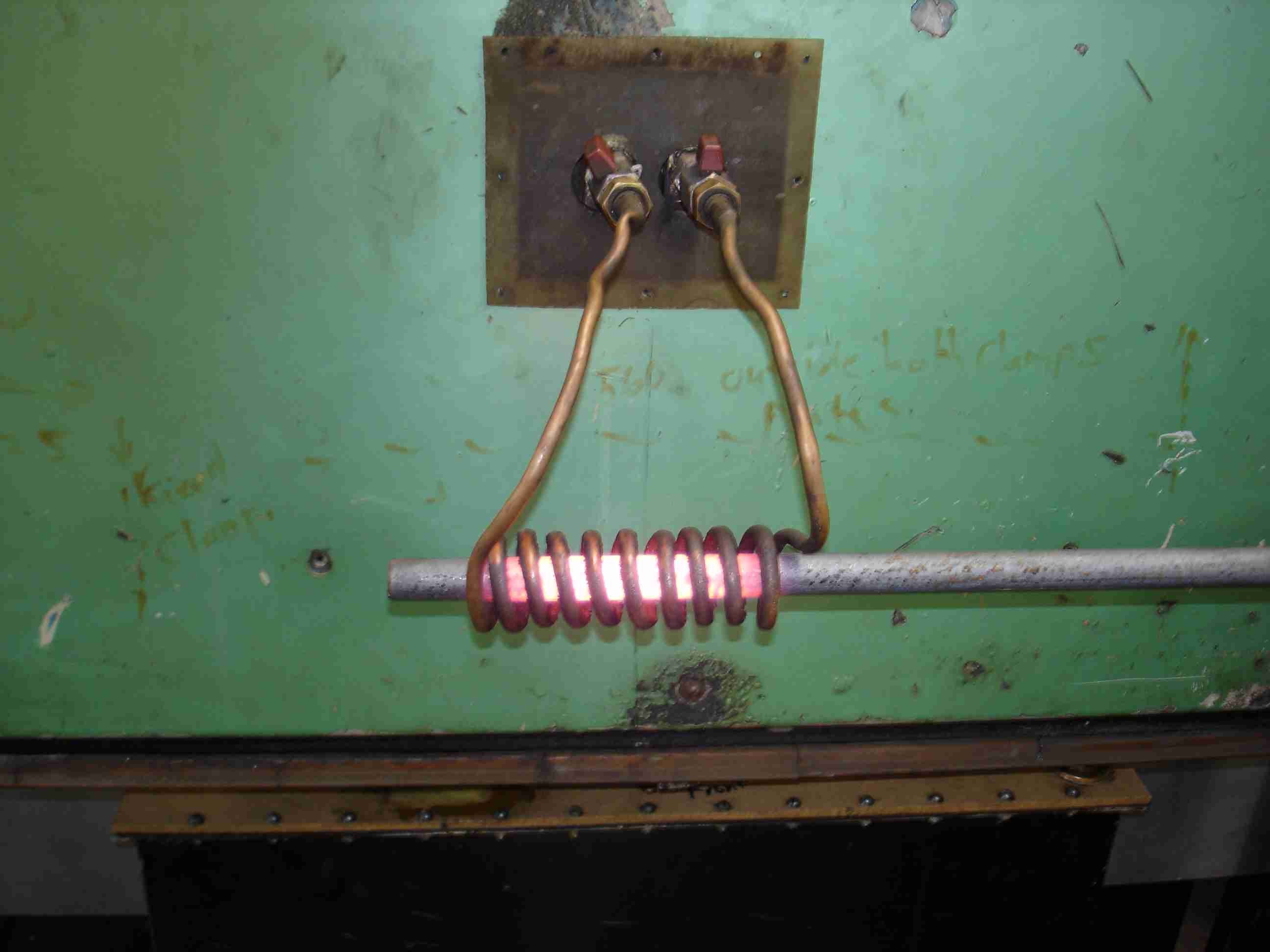
Real-world examples of this are everywhere: the heating element inside a soldering iron, or resistance heating wires in an electric blanket. As electric current flows through metal, heat is generated uniformly throughout the rod. The operating condition I envisioned is: the left end of the rod is clamped to a cooling base at 350 K (about 77 °C), while the right end is exposed to ambient air at 300 K (about 27 °C) for natural convective cooling. A typical heat conduction experiment looks something like this: heating a metal rod with a candle, placing temperature sensors along the rod, and acquiring data with an Arduino.

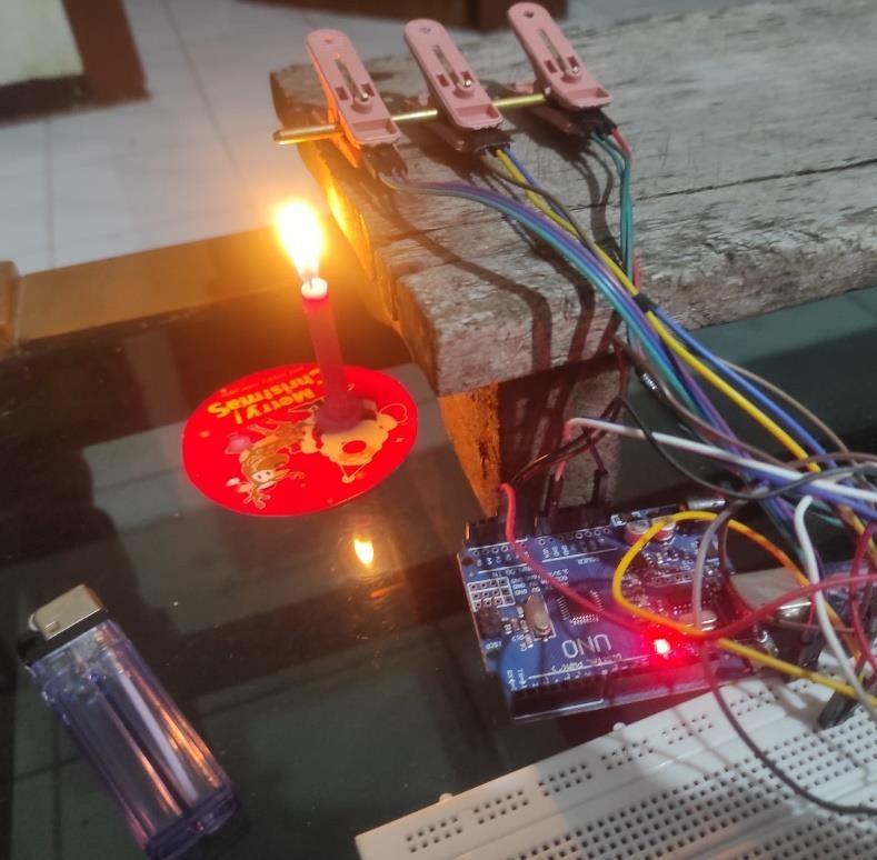
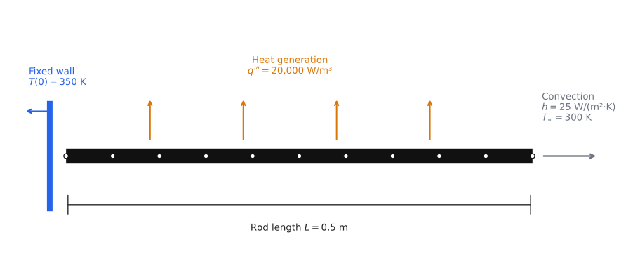
I simplified the model to uniform internal heat generation across the entire rod, with heat conducted through the metal due to temperature gradients and exchanged with the environment at the boundaries. The model parameters are as follows:

• Rod length $L = 0.5$ m, thermal conductivity $k = 167$ W/(m·K) (typical aluminum alloy scale)
• Uniform volumetric heat generation $q''' = 20{,}000$ W/m³
• Left boundary fixed at $T_{\text{left}} = 350$ K
• Right boundary ambient air $T_\infty = 300$ K, heat transfer coefficient $h_c = 25$ W/(m²·K)

I wanted to know: where is the hottest point along the rod, how much heat escapes from each end, and more importantly—can the code I wrote actually be trusted?

Deriving an Analytical Benchmark First

Before writing any code, derive a benchmark solution by hand. The steady-state 1D heat conduction equation is:

$$k\frac{d^2T}{dx^2}+q'''=0,$$

with a Dirichlet temperature condition on the left and convective cooling to the air on the right:

$$T(0)=T_{\text{left}},\qquad -k\frac{dT}{dx}\bigg|_{x=L}=h_c\left[T(L)-T_\infty\right].$$

This equation is straightforward. Integrating twice yields the general temperature profile:

$$T(x)=T_{\text{left}}+C_1x-\frac{q'''x^2}{2k},$$

The integration constant $C_1$ is determined by the convective boundary condition at the right end. Substituting the parameters yields the exact benchmark solution: a right-end temperature of 360.446 K, and a maximum temperature of 360.788 K occurring at $x\approx0.4244$ m. Later, when checking the code, these values and the entire analytical curve serve as the ground truth.

Discretizing the Rod into a Grid

The governing equation is continuous, but computers only operate on discrete numbers, so we first discretize the rod into a computational mesh. The rod is divided into $N$ equal segments of spacing $h=L/N$. Interior nodes use standard central differencing, where each node interacts only with its immediate left and right neighbors:

$$\frac{k}{h^2}\left(T_{i-1}-2T_i+T_{i+1}\right)=-q'''_i.$$

The left boundary is simple: with temperature prescribed, we directly set $T_0=T_{\text{left}}$. The right boundary is where the real trap lies: the surface node sits at $x=L$, backed by only half a control volume. Its energy balance must account for three distinct terms: heat conducted from the interior, heat generated within this half-cell, and heat carried away by convection into the ambient air:

$$\frac{h}{2}q'''_N =h_c(T_N-T_\infty).$$

The middle term—heat generated in that half-cell—is the easiest to overlook. If omitted, the resulting temperature curve still looks smooth and plausible, but the overall energy balance will no longer close—exactly the kind of silent, seemingly harmless error I was concerned about from the start.

Implementing the Solver

Assembling the equations for all nodes produces a tridiagonal matrix system: all entries are zero except along the main, upper, and lower diagonals. This system can be solved efficiently using the Thomas algorithm (tridiagonal matrix algorithm, TDMA), which performs a forward elimination pass followed by a backward substitution pass. Its computational cost scales linearly with the number of nodes. Rather than calling an off-the-shelf NumPy solver, I implemented the algorithm from scratch. The full solver implementation is on GitHub: src/steady_conduction_1d.py, where assemble_system builds the linear system and thomas_solve solves it.

With the solver completed, we arrive at the core question of this article: is it actually correct? I validated it across four distinct dimensions.

1. Comparison with the Analytical Benchmark

Once the code ran, I performed grid refinement as textbook guidelines suggest: setting $N$ to 20, 40, 80, and 160 to observe how the error relative to the analytical solution drops. When the results came out, I was initially thrilled: at $N=160$, the maximum error was only $1.34\times10^{-11}$ K—unbelievably small. But the more I thought about it, the more suspicious it seemed. Why would the error be so tiny?

Revisiting the mathematical derivation revealed why: the exact solution to this problem is a second-order polynomial, whereas the leading truncation error of central differencing is proportional to the fourth derivative of temperature. The fourth derivative of a quadratic curve is identically zero, meaning central differencing is exact for this specific problem with zero discretization error. The measured $1.34\times10^{-11}$ K was not discretization error at all, but merely floating-point roundoff noise. Thus, this initial check only proved half of what was needed: the matrix assembly and boundary conditions were implemented correctly, but the theoretical convergence order had not been tested at all.

2. Does the Error Decay at Second Order?

To verify the order of accuracy, we need a problem that central differencing cannot solve with zero truncation error. I applied the Method of Manufactured Solutions (MMS): first defining an arbitrary temperature profile with a sinusoidal curvature:

$$T_m(x)=T_{\text{left}}+C_1x+A\sin\left(\frac{\pi x}{L}\right),\qquad A=8\ \text{K},$$

and then substituting it back into the governing equation to derive the exact source term required to sustain this profile:

$$q'''(x)=kA\left(\frac{\pi}{L}\right)^2\sin\left(\frac{\pi x}{L}\right).$$

The fourth derivative of a sine function is non-zero, so truncation error is unavoidable. Repeating grid refinement under identical boundary conditions:

Element Count $N$	Grid Spacing $h$	Max Nodal Error
20	0.025 m	$4.81\times10^{-2}$ K
40	0.0125 m	$1.20\times10^{-2}$ K
80	0.00625 m	$3.00\times10^{-3}$ K
160	0.003125 m	$7.51\times10^{-4}$ K

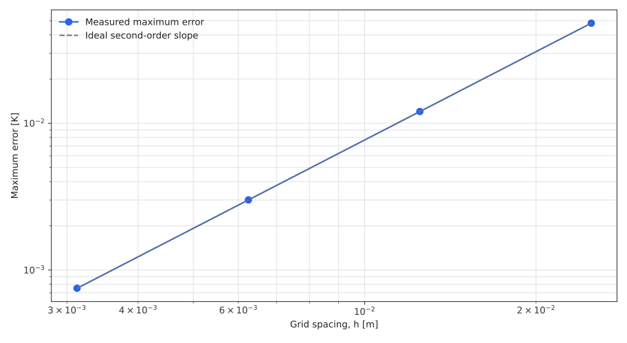
Each time the grid spacing is halved, the error decreases by a factor of four, following an exceptionally clean trend. The fitted convergence order is 2.0002, falling well within the expected 1.8–2.2 range and confirming formal second-order spatial accuracy.

3. Global Energy Conservation

With the convergence order confirmed, the next step is verifying global energy conservation: the total heat generated inside the rod must exactly equal the heat conducted out the left boundary plus the heat convected away at the right boundary. The total heat generated per unit cross-sectional area across the rod is 10,000 W/m², with 8,489 W/m² conducted out through the left boundary and 1,511 W/m² dissipated through the right boundary. Across three grid refinements, the relative residual remained below $1.59\times10^{-12}$—confirming that the numerical model neither leaks nor creates artificial heat at the boundaries.

4. Verification of the Linear Solver

The previous three checks all rely on an underlying assumption: that the assembled linear system was solved correctly. That assumption rests entirely on the hand-written Thomas algorithm implementation, which had not yet been independently verified.

Using a fixed random seed, I generated 64 random $64\times64$ tridiagonal systems and solved each using both my Thomas solver and numpy.linalg.solve. Across all test cases, the maximum discrepancy was only $1.1\times10^{-16}$, well within machine precision. Coupled with unit tests checking dimension mismatches, zero-pivot detection, and linear temperature degeneration in the absence of heat sources, the solver implementation itself was proven robust.

At this point, all four validation pillars were fully satisfied: equation assembly, discretization accuracy, boundary energy conservation, and linear solver correctness. Now we can return to the initial engineering questions.

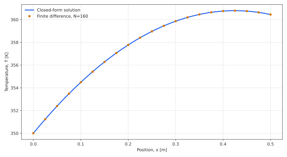
The peak temperature does not occur at either endpoint, but inside the rod at $x\approx0.42$ m, reaching approximately 361 K (around 88 °C); the right endpoint is slightly cooler at around 360 K. Both values match the analytical benchmark (360.788 K and 360.446 K) with high fidelity.

The physical reason why the peak is not at the boundary is straightforward: convective heat dissipation to the ambient air on the right is relatively weak, so heat cannot escape fast enough and accumulates near the right end. However, the heat distribution pathways are somewhat counterintuitive: of all the heat generated within the rod, roughly 85% is conducted away through the left cooling base, while only about 15% is dissipated into the air from the right end. In other words, the rod is primarily cooled by conduction into the left base, rather than convection from the surrounding air.

Summary

Looking back on this verification exercise, my key takeaway is that small error does not necessarily mean the method is verified. Seeing an error of $10^{-11}$ initially led me to believe everything was working, but that was merely an illusion caused by the degenerate simplicity of the test problem.

Furthermore, a complex verification problem is best decomposed into targeted checks that each isolate a specific mechanism: an analytical benchmark verifies equation assembly, a manufactured solution tests convergence order, an energy balance verifies global conservation, and independent unit tests verify the linear solver. In subsequent projects—such as a 2D transient thermal diffusion solver, or cooling calculations for electric motor water jackets and inverter cold plates—I consistently applied this modular verification strategy. The ~85% to 15% heat split in this 1D case also reinforced an engineering habit: solve the 1D case first before deciding whether to introduce more complex multidimensional models.

Finally, the physical assumptions and boundaries of this model must be clearly stated: it assumes 1D steady-state conduction with constant material properties, neglecting contact resistance, thermal radiation, and temperature-dependent properties; the manufactured solution serves purely as a mathematical verification tool rather than an operational condition. What it proves is that, under these assumptions, the governing equations, spatial discretization, and code implementation are completely self-consistent.

Code

All solver code, test suites, and plotting scripts for this project are open source: gaoflow/steady-conduction-1d

Local commands:

git clone https://github.com/gaoflow/steady-conduction-1d.git
cd steady-conduction-1d
python3 -m unittest discover -s tests -v
python3 scripts/analyse.py